Welcome to Part 2 of this series! Now that we understand the concept of Stereo Vision (Part 1), let’s finally move on to creating our depth map.
Let’s start this camera!
All the scripts we will be using for this tutorial are written in Python.
To get started, clone my StereoVision repository.
Requirements
If you have not set-up your Jetson Nano yet, please visit this site.
Assuming that you have got your Jetson Nano up and running, let’s install all the requirements for this project.
Since we are going to be working on Python3.6, let’s install
pip for Python3 : sudo apt-get install python3-pip
Python3.6 development packages: sudo apt-get install libpython3-dev
Then install all other requirements: pip3 install -r requirements.txt
If you wish to install the requirements manually, you could type:
Install cython: pip3 install cython
Install numpy: pip3 install numpy
Install StereoVision library: pip3 install StereoVision
Side Note: If you face any errors during this project, please head to the Troubleshooting section of my repo.
Testing the Cameras
Before creating a proper enclosure or a temporary stand for our Stereo Camera, let’s test if the cameras turn on.
For now, you can plug in the two Raspberry Pi cameras and test whether they run upon entering these terminal commands:
# sensor_id selects the camera: 0 or 1 on Jetson Nano B01
$ gst-launch-1.0 nvarguscamerasrc sensor_id=0 ! nvoverlaysink
Try this for sensor_id= 0 and 1 to test if both cameras work.
If you face a GStreamer error like such:

Type sudo service nvargus-daemon restartin your terminal and try again.
Sometimes the Gstreamer pipeline may not be closed properly upon quiting a program. Therefore,this command comes in very handy (something you should remember) 😃!
If the issue persists, then ensure the cameras are plugged in properly and restart the Jetson Nano.
Fixing the Pink Tint
If you realise a slight pinkish tint in your camera, please follow these steps from Jonathan Tse.
Getting the hardware setup ready
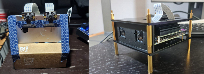
Before we move any further, we must have a stable Stereo Camera with the two Raspberry Pi lenses placed a fixed distance apart (this is the baseline).
It is important to keep the baseline fixed at all times. I found a 5cm baseline to be optimal, but you could try different separation distances and drop a comment on your results!
There are many ways to do this, so use your imagination!

Initially, I used BluTac to stick the cameras to an old iPhone and the Jetson Nano box.
I decided to use onShape and design a simple 3D CAD Model. I then used a Laser Cutter and cut out the pieces from Acrylic, resulting in the dog-like enclosure you see on the right 😜!
If you are interested to see the model, you can view my CAD Design!
If you would like to design your own CAD model, you can download the 3D STEP model from here.
Starting the Cameras
Now that we have ensured that our cameras are connected properly, let’s start them.
To run the Python scripts, navigate to the/StereoVision/main_scripts/directory in the terminal.
Run the start_cameras.py script: python3 start_cameras.py
You should see the live video feed from both your cameras side-by-side.
If you face any errors starting the camera, visit this page.
Let’s get that ChessBoard ready!
I will be using a 6x9 (rows x columns) chessboard for this project. You can get the image from my GitHub repository, or if you have already cloned it then you have the file!

Print out the picture (make sure not to fit-to-page or change the scaling) and stick the image onto a hard surface (such as a clipboard or a box).
The easiest way would be to use this image of the Chessboard that I have provided. However, if you do wish to use your own Chessboard, make changes to the 3_calibration.py on lines 16 and 19.
Taking Pictures
We will be taking 30 images at 5-second intervals.
Suggestions
- Don’t stand too far away. Make sure the Chessboard is covering the majority of the camera frame.
- Make sure to cover all corners of the frame.
- Make sure to move and rotate the Chessboard between images to get pictures from different angles.
Move the chessboard slightly between each picture but ensure you do not cut out part of the image. Images from both cameras will be stitched together and saved as a single file.
To take pictures, type python3 1_taking_pictures.py
If you face an error when trying to start the cameras saying: Failed to load module “canberra-gtk-module”…
Try this:
sudo apt-get install libcanberra-gtk-module
If you wish to increase the time interval between pictures or the total number of pictures taken, modify the 1_taking_pictures.py script. The Photo Taking Presets are right at the top.
If you want to stop any Python program from this series, press Q on your keyboard.
You should now have a new folder called “images” with all the pictures you just took saved in it!
Accepting/Rejecting and Splitting the pictures.
To ensure that we don’t use poor quality images (missing parts of the chessboard, blurry, etc.) for the calibration, we will go through every picture taken and ACCEPT or REJECT it.
To do this, let’s run python3 2_image_selection.py
Run through all the images. Press ‘Y’ to save the image and ‘N’ to skip.
Now, the Left Camera and Right Camera images will be saved separately in the folder called ‘pairs’.
Calibration Time!
This is an extremely important step in this series. It is essential for us to rectify and calibrate our cameras to obtain a desirable disparity map.
Thanks to Daniel Lee’s Stereo Vision library, we don’t have to do much in terms of the code!
To do the calibration, we will run through all the Chessboard images you saved in the previous step and calculate correction matrices.
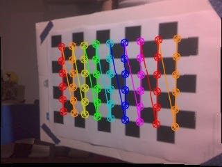
The program will do the Point-Matching process and try to find the Chessboard corners. If you feel the results are inaccurate, try retaking your pictures.

To do this, let’s run: python3 calibration.py
After running through all the image pairs, give the program some time to calibrate the results (about 1–2 minutes).
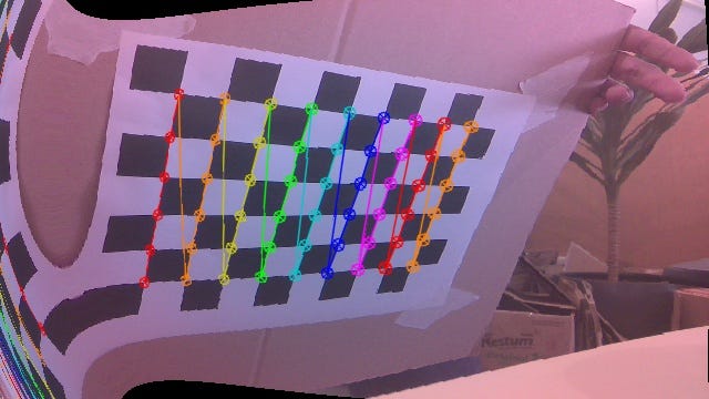
Once complete, you will see the calibration results — the rectified images.


If your calibration results look slightly wonky (like those above), you can try to redo Steps 1–3.
Your rectified images will never look perfect, so don’t be afraid of the results and continue to the next step!
You can always come back!
Tuning the Disparity Map!

Now that our cameras are ready to go, let’s start tuning the disparity map itself!
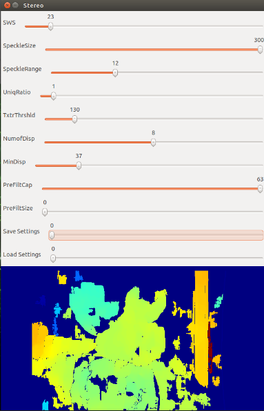
Run 4_tuning_depthmap.py: python3 4_tuning_depthmap.py
To understand the Variables — check the ReadME file on my GitHub repo.
The ranges on the tuning bars may slightly differ from those listed in the explanations. This is because I had to modify the parameters shown on the GUI due to the limitations of OpenCV’s trackbars.
With the tuning window, you will also see your left and right rectified images side by side in grayscale. This is for you to compare your Depth Map to and know what to expect.
Finally…The Depth Map!
All steps are complete!
We can finally run 5_depthmap.py: python3 5_depthmap.py
And there we have it, a fully functional depth map that we created from scratch!
Determining the actual distance to objects
The depth map you see above in (5_depthmap.py) is a 2-dimensional matrix. So why not get the actual depth information from it!
To determine the distance to a specific object in the frame, click on it to print the relative distance in Centimeters to the terminal. By doing this, you are actually determining how far the specific pixel is from the camera.
What this distance really means
Now one thing to understand is, the distance measured is not the exact distance away from the center of the camera system, but the distance away from the system in the Z-axis.

Therefore, the distance we are actually measuring is y and not x.
It’s not over yet
A depth map is cool. But Terminators also need to be able to detect people before they attack.
Check out Part 3 to add Object Detection capabilities to this depth map, allowing us to determine the relative distance of a person from the camera!
